


IFundamentals of Thermal Design
1.1Core Theory and Formulas
Thermal resistance model: switched-mode power supply thermal design is based on a series thermal resistance (°C/W) model; the total thermal resistance path is:
- Rj_a
- total junction-to-ambient thermal resistance (°C/W)
- Rj_c
- junction-to-case thermal resistance (°C/W)
- Rc_s
- case-to-heatsink interface thermal resistance (°C/W)
- Rs_a
- heatsink-to-ambient thermal resistance (°C/W)
Junction temperature calculation formula:
Design rule: the junction temperature of key components should be at least 20% below the rated value; for example, a MOSFET rated at 150°C should have a design target of ≤120°C
This article only covers cooling for heat dissipation below 500W (corresponding to power supplies below 5KW). For units dissipating more than 500W, heat pipes and liquid cooling systems are used and are omitted here.
1.2Temperature Rise vs. Lifetime
Industry rule of thumb: for semiconductors, electrolytic capacitors, inductors and transformers, every 10°C rise in internal temperature halves their service life. (Note: this rule does not hold for other types of components such as resistors and film capacitors.)
Electrolytic capacitor lifetime formula:
where T is the capacitor temperature (in general the surface temperature differs little from the internal temperature)
Tmax is the rated temperature (usually 105°C)
L_Tmax is the rated lifetime of the electrolytic capacitor at the rated temperature (see datasheet)
IICooling Method Selection and Scheme Design
2.1Natural Convection and Radiation Cooling Calculation without a Fan
- Principle
- cooling relies on natural airflow generated by the density difference between cold and hot air
- Applicability
- power chargers with low power density (typical standard <0.5W/cm³); for highly efficient supplies with uniform internal heat conduction, this can be relaxed to <0.8W/cm³
Design points and calculation methods:
2.1.1Heat Dissipation and Surface Temperature of a Closed Body (e.g. Power Adapters)
- Physical model and assumptions
Typical scenario: a plastic/metal enclosure (e.g. charger, adapter) lying flat on a desk
Three prerequisite assumptions:
- The enclosure surface temperature is uniform
- The ambient temperature is constant
- The desk is an adiabatic surface (in reality there is slight conduction, negligible in conservative calculation)
- Heat dissipation paths are natural convection + radiation from the top surface and four side surfaces (the surface touching the desk is ignored)
Natural convection heat dissipation power Pconv formula:
where h_up and h_side are the convection heat transfer coefficients of the enclosure top and side surfaces,
Aup and Aside are the areas of the enclosure top and side surfaces
ΔT is the difference between the enclosure surface temperature and the ambient temperature (i.e. the enclosure temperature rise)
h_up = Nu_up*k_air/L, where Nu_up is the Nusselt number correlation for the top surface:
g is the gravitational acceleration, 9.8
β coefficient, taken as 1/(T_s/2+T_2+273)
L is the characteristic length; for side surfaces it is the height
v is the air viscosity, 1.56*10-5 at 25°C
Pr is the Prandtl number, 0.71 for air at 25°C
k_air is the air thermal conductivity, 0.026W/(m*K) at standard room temperature
L is the characteristic length; for side surfaces it is the height, in m
h_side = Nu_side*k_air/L, where Nu_side is the Nusselt number correlation for the side surface:
Similar to h_up, but the characteristic length L is computed differently; for the top surface:
L=area/perimeter=a*b/2*(a+b),
Radiation heat dissipation power Qconv formula:
ε surface emissivity: 0.9 for plastic enclosures, 0.85 for anodized aluminum, 0.3 for bare metal
σ Stefan-Boltzmann constant, 5.67*10-8
Ts is the enclosure surface temperature, Ta is the ambient temperature, in absolute temperature K
Engineering simplification (Ts in the 50~80°C range, error <5%)
For quick engineering evaluation, a rough empirical formula can also be used (error ±15%):
h_eff composite coefficient: 8~10 for plastic enclosures, 10~12 for anodized aluminum, 6~8 for others
2.1.2Calculation example: a power supply with a black plastic enclosure, 114*69*29mm, total heat dissipation 10W
By this rough formula, the enclosure temperature rise is 54°C
Taking ε = 0.9, Atotal has been computed as 0.01848
Next calculate the convection heat Qconv
h_up = Nu_up*k_air/L,
L = 0.029, other parameters same as h_up
= 9W
Conclusion: with a 50°C temperature rise, this enclosure can theoretically dissipate 13W of heat.
2.1.3Notes
Note that the above calculation assumes no heat dissipation from the bottom. In reality the enclosure bottom touches the desk and can also dissipate some heat. If 1~2mm standoff bosses are added under the enclosure, a micro-circulation air convection layer forms at the bottom; with the same enclosure temperature rise, this 1~2mm bottom air layer helps raise the heat dissipation by 10~15%.
Note that another important assumption of the above calculation is a uniform enclosure surface temperature. In design, measures should be taken to equalize the internal surface temperature of the enclosure, such as potting with low-thermal-resistance thermally conductive glue, or pressing highly conductive copper or aluminum tightly against the inner walls.
For quick rough evaluation, use the empirical formula Qtotal = h_eff *Atotal*ΔT; for more precise calculations, use the more complex formula Qtotal = Qconv + Qrad.
A very important point: the theoretical formulas above also come from big-data fitting of engineering practice; their results deviate somewhat from real measurements and serve as theoretical references at the design stage. In actual engineering application, verify in detail with experimental data, and if necessary revise, supplement and refine some coefficients of the empirical formulas above.
2.2Forced-Air Convection Cooling Calculation with a Fan
Here we assume a rectangular power supply model, sealed on all sides, with air intake on one side and exhaust on the other
Fan selection formula:
where ρ is the air density (1.18kg/m³), cp is the specific heat capacity (1005J/kg·K),
ΔT is the temperature rise (difference between the incoming cold air and outgoing hot air), generally 10-15°C
Vrequired is the required fan airflow
Example: power supply enclosure 265*134*60mm, total internal heat 100W, how to select the fan?
First calculate the external natural convection and radiation dissipation of this enclosure
Since forced-air cooling dominates here, the natural dissipation from the enclosure surface is auxiliary and can be estimated with a simple empirical formula:
ΔTs is the temperature difference between the enclosure surface and the ambient; we tentatively set 25°C
This dissipation is only 1/5 of the target.
Forced-Air Cooling
ρ=1.18
Electronic fans commonly use the CFM unit (cubic feet per minute). Its conversion with standard
In general, the nominal airflow of an electronic fan is the 'free air flow'. After being installed in a power supply, the real measured airflow is only 0.4~0.7 of the nominal value due to airflow resistance. When the resistance is unknown, take the attenuation as 0.5. Therefore, for this case an 18CFM fan satisfies the design requirement.
- Conclusion
- for this enclosure case, a fan with airflow greater than 18CFM preliminarily meets the temperature rise design requirement. The specific structure needs experimental verification.
- Verification
- for the G1200 power supply, output 1200W, heat 100W, fans are 4028,
speed 16000, airflow 22CFM. This example uses two 4028 fans, theoretical
airflow 44CFM, far above the 18CFM requirement. In principle one fan would suffice; we need to examine why it was designed this way.
Key Points of Airflow Duct Design with Fan Cooling
Airflow duct design is the 'last mile' that determines cooling success. A good design can raise
cooling efficiency by 50% and cut noise by 10dB; a poor design creates 'heat islands' even with the right fan.
Overview of core principles:
Essence of duct design: within limited space, guide cold air to flow 100% through the heat sources with minimal pressure loss, and exhaust the hot air quickly.
Three red lines:
Intake area ≥ exhaust area × 1.2 (prevents negative pressure sucking in dust)
Duct resistance < fan maximum static pressure × 60% (prevents stall)
Dead-flow area < 5% of total volume (prevents local overheating)
Four Rules of Airflow Organization
- Rule 1
- Prefer bottom-in top-out; secondarily, opposite-side in/out.
- Principle
- hot air is less dense (~1.1kg/m³) and rises naturally, while cold air is denser (~1.2kg/m³) and sinks. Bottom-in top-out adds natural convection, boosting total airflow by 10-15%.
- Intake location
- bottom or lower side of the enclosure, ≥10mm above the desk
- Exhaust location
- top or upper side of the enclosure, placed diagonally opposite the intake
- Taboo
- intake and exhaust on the same or adjacent side — short-circuit rate >50%
- Rule 2
- Keep the duct cross-section constant or gradually expanding; avoid abrupt cross-section changes
Per the Bernoulli equation, abrupt cross-section changes cause static pressure loss and significant airflow decay.
Rule 3: Heat sources must be inside the duct and aligned with the airflow direction
Place heat-generating components parallel to the duct, avoid perpendicular mounting, and position the largest heat sources near the intake.
- Rule 4
- Eliminate airflow dead zones
- Add guide vanes
- 45° chamfers at corners to reduce turbulence
- Fin alignment
- heatsink fins face the exhaust directly, deviation <5°
- Fill cavities
- seal gaps in the duct with foam or partitions to prevent airflow 'shortcuts'
Several details need attention:
- Vent hole open-area ratio and shape:
The recommended open-area ratio (vent area/enclosure surface area) is 20-30%. If <15%,
airflow resistance is high and airflow insufficient. If >40%, EMI shielding weakens, enclosure strength drops,
and the EMI metal shielding function is greatly reduced.
Also, even at the same open-area ratio, different hole shapes give different airflow resistance:
Hole shape comparison (same open-area ratio); honeycomb hexagon holes are the first choice:
| Shape | Air Resistance | EMI Shielding | Dust Clogging | Recommendation |
|---|---|---|---|---|
| Round holes (Φ3mm) | Medium | Good | Easy | ★★★★★ |
| Hexagonal honeycomb | Low | Excellent | Medium | ★★★★☆ |
| Louvers | Very Low | Poor | Very Hard | ★★★☆☆ |
| Long Slots | Low | Poor | Medium | ★★☆☆☆ |
If round-hole arrays are chosen: hole diameter 3-5mm, hole pitch 8-10mm, plate thickness 0.8-1mm
- Blow or exhaust (conclusions only; engineering analysis omitted)
- Fan mounting position: the fan should be 5-10mm from the heatsink or hot plate. Too far causes airflow diffusion; below 5mm adds about 5dB of local turbulence noise.
- Minimize airflow resistance and duct pressure loss. When duct pressure loss exceeds 60% of the fan pressure, the fan enters the nonlinear region and airflow plummets.
The engineering calculation is very complex; in practice adjust the design with actual pressure measurements. Use a micromanometer to measure the pressure difference across the fan; it should be kept below 70% of the rated static pressure.
A simple theoretical calculation is also given for reference:
ΔPfriction frictional resistance along the path (Darcy-Weisbach formula):
f is the friction factor (64/Re, where Re is the Reynolds number)
L is the characteristic duct length (m)
p is the air density, 1.2Kg/m3
v is the air velocity (m/s)
ΔPlocal is the local resistance:
K coefficient: 1.1~1.5 for 90° elbows
0.3~0.4 for 45° bends
- In high-altitude regions, e.g. 2000m elevation, air density drops 18%; the same fan moves the same airflow volume but its cooling capability drops 18%.
2.3Heatsinks and Related Thermal Calculations
3.3.1Introduction to Heatsinks
- Structure types:
- Pin-fin heatsinks
- isotropic, suitable for irregular spaces
- Plate-fin heatsinks
- highly directional, must align with the airflow direction
- Grooved heatsinks
- increase surface area by 30%, suitable for duct design
- Material selection:
- Aluminum (6063)
- thermal conductivity 205W/(m·K), cost-effective
- Copper
- thermal conductivity 401W/(m·K), heavy and expensive
- Thermal interface materials:
| Material Type | Thermal Conductivity | Thickness | Thermal Resistance | Application |
|---|---|---|---|---|
| Thermal grease | 5-10 W/(m·K) | 5-20μm | 0.05-0.2℃/W | Enclosure-metal tight contact |
| Thermal pad | 2-5 W/(m·K) | 0.5-1mm | 0.2-0.5℃/W | Filling 0.1-0.5mm gaps |
| Phase-change material | 3-8 W/(m·K) | 0.05-0.2mm | 0.1-0.3℃/W | Softens and fills at high temperature |
| Insulating silicone sheet | 1-3 W/(m·K) | 0.15-0.3mm | 0.5-1℃/W | Electrical insulation applications |
| Mica sheet | 0.7 W/(m·K) | 0.1mm | 1-2℃/W | High-voltage insulation |
- Fin design:
- Thickness
- 0.5-1.5mm (aluminum); too thin lacks strength, too thick adds weight
- Pitch
- ≥6mm for natural convection, 3-5mm for forced-air cooling
- Height
- doubling the height only reduces thermal resistance by about 30% (diminishing returns)
- Count
- too many fins obstruct airflow; optimize with CFD simulation
- Base plate thickness:
- Die-cast aluminum
- ≥3mm (ensure strength)
- Extruded aluminum
- ≥2mm
- Skived-fin process
- 1-1.5mm (fins and base formed integrally)
- Surface treatment:
Anodizing: after blackening, emissivity ε rises from 0.05 to 0.85
3.3.2Heatsink Dissipation Power and Temperature Calculation with Natural Convection Only
Without a fan, the heatsink dissipation power is calculated as in the following example:
With the above premises, the heatsink-to-ambient thermal resistance Rs_a can be calculated as follows
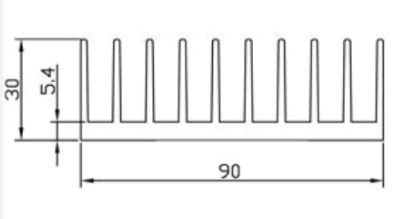
You can also use the formula in Section 3.1 (Qtotal = h_eff *Atotal*ΔT) to roughly calculate the dissipation power of a natural-convection heatsink,
for example, an aluminum profile heatsink with cross-section as shown at lower right:
length, width and height are 90*30*40mm,
mounted vertically on the PCB,
it has 10 fins, 2 surfaces each,
Rough dissipation power Qtotal = h_eff *Atotal*ΔT,
taking Qtotal as 1.0, the computed ΔT is the thermal resistance,
Interpretation: this heatsink has a thermal resistance of 4.8°C/W; conducting 10W into it raises its surface temperature by 48°C
Note: in fanless scenarios relying only on natural convection, heatsink fin spacing must be ≥6mm; if too small, cold air can hardly enter between fins to exchange heat. With forced-air cooling, fin spacing should still be greater than 3mm.
2.3.2Heatsink Dissipation Power and Temperature Calculation with Forced Air
Under forced-air cooling, air heat transfer is directly determined by the fan air velocity u; radiation accounts for less than 5% and is negligible.
u is the air velocity in m/s,
b is the velocity exponent: 0.5 below 2m/s,
L is the fin length along the duct
η is the fin correction factor, generally 0.6~0.8
A is the total fin area exposed to the flowing air
Interpretation: at 4m/s air velocity, this heatsink has a temperature rise of 55°C with 50W of heat
Note: fans are generally rated by airflow (in CFM). The relationship between airflow and velocity is: V = u*A, where V is airflow, u is air velocity, A is the duct cross-sectional area.
Fan airflow V= 4*0.0027 = 0.0108 m3/s = 22 CFM.
2.3.3Cooling Fan Parameter Selection
The key to selecting an electronic cooling fan is understanding the true physical meaning of the three main parameters — airflow, static pressure and noise — and how they match the system impedance. Looking at any single parameter alone can fall into the 'paper performance' trap. The core three parameters are airflow, static pressure and noise; other details are described below:
1Airflow (CFM / m³/h) — 'the capacity to move air'
- Test condition
- the maximum measured in free air (no resistance); it inevitably decays after actual installation.
- Applicable scenarios
- open ducts, whole-chassis ventilation, low-resistance environments. For dense-fin heatsinks, the nominal CFM is of greatly reduced reference value.
- Key insight
- more airflow is not always better; effective airflow must be assessed together with static pressure.
2Static pressure (Pa or mmH₂O) — 'the push to penetrate resistance'
Definition: the pressure difference a fan can generate when overcoming system resistance (fins, filters, duct bends). 1 mmH₂O ≈ 9.81 Pa.
Applicable scenarios: high-resistance environments such as heatsinks, dust filters, sealed cavities. High-static-pressure fans can 'squeeze' air through narrow gaps. Relationship with airflow: inversely proportional. The PQ curve shows that the higher the static pressure, the smaller the actual airflow; at zero static pressure, airflow reaches its maximum (free air flow).
Engineering experience: server heatsinks are recommended to have static pressure ≥ 3 mmH₂O; industrial VFDs need ≥ 5 mmH₂O.
3Noise level (dBA) — 'subjective listening comfort'
- Definition
- A-weighted sound pressure level, simulating the human ear's sensitivity to different frequencies. Every +3 dBA ≈ sound power ×2; +10 ≈ perceived loudness doubled.
- Measurement conditions
- must be measured at 1m distance, in a semi-anechoic chamber, at rated speed; otherwise the value is meaningless.
- Spectrum trap
- two fans both at 30 dBA — low-frequency 'hum' is more annoying than high-frequency 'hiss'. Pay attention to the spectral distribution.
- Noise sources
- bearing friction, blade turbulence, motor electromagnetic noise, etc. Ball bearings are noisier than fluid dynamic bearings but last longer.
Note: after the fan is installed in equipment, the noise generated by airflow resistance may greatly exceed the fan's own noise.
4PQ curve (performance curve) — the 'decision map' for selection
- Essence
- a measured curve with airflow Q on the horizontal axis and static pressure P on the vertical axis, reflecting fan performance under real resistance.
- Operating point
- the intersection of the fan PQ curve and the system impedance curve is the actual operating condition. The system impedance curve is a quadratic parabola; resistance ∝ airflow².
- Selection strategy
- prefer the middle-right region of the PQ curve where efficiency is highest.
The more 'square' the curve (pressure does not collapse quickly in the high-pressure region), the better the dust resistance
5Bearing type — the trade-off between lifetime and noise
| Bearing Type | Lifetime (h) | Noise | Orientation Sensitive | Cost | Application |
|---|---|---|---|---|---|
| Sleeve bearing | 20k–30k | Low | Sensitive | Low | Horizontal mounting, light load, low cost |
| Ball bearing | 50k–80k | Medium | Insensitive | Medium | High speed, industrial equipment |
| FDB / fluid dynamic | 80k+ | Very Low | Insensitive | High | Silent PCs, medical equipment |
Note: mounting a sleeve bearing vertically or upside-down accelerates lubricant loss, halving lifetime
6Lifetime metrics (L10/MTBF) — temperature is the invisible killer
- L10
- the time point at which 10% of fans fail, usually @25°C or 40°C.
- Rule of thumb
- for every 10°C rise in ambient temperature, lifetime drops by about 30–50%. The L10 lifetime at 50°C is only 1/3 of that at 25°C.
- Closed-loop feedback
- fans with a Tach signal enable speed monitoring and fault alarms.
7Input power and efficiency: airflow per watt (CFM/W) is the core energy-efficiency metric. A fan with high CFM but huge power consumption is not cost-effective. The electrical power consumed by the fan itself turns into heat, which in enclosed spaces can backfire on cooling performance.
- Four-Step Selection Method (System Perspective)
- Step A
- Determine the system resistance level
- Low resistance
- large open areas, short straight ducts → prefer high-airflow types (e.g. chassis exhaust)
- Medium resistance
- conventional heatsinks, dense fins → balanced types
- High resistance
- dust filters, HEPA, serpentine ducts → high-static-pressure types are required (e.g. server CPU coolers)
- Step B
- Lock in size and speed
- Size first
- at the same speed, a 120mm fan is 3–5 dBA quieter and over 40% higher in airflow than an 80mm fan. Use the largest size possible.
- Step C
- Compare the PQ curve with the system impedance
No system curve? Estimate resistance from open-area ratio, filter grade and duct length, and choose a model that maintains usable airflow in the medium-high pressure region.
- Measurement method
- measure the system impedance with the two-chamber method or a wind tunnel; intersect with the PQ curve to get the actual airflow.
- Step D
- Verify noise and energy efficiency
Check dBA and CFM/W at the target operating condition. If necessary, choose a PWM speed-controlled fan to balance full load and standby.
9Practical Comparison and Misconceptions
Case: compact fin heatsink with a medium-density filter (medium-resistance system)
Fan A (high airflow / low static pressure): nominal 80 CFM / 1.2 mmH₂O, actual operating point drops to 40 CFM, noise 32 dBA
- Fan B (balanced / high static pressure)
- nominal 70 CFM / 2.8 mmH₂O, reaches 55 CFM in the same system, noise 33 dBA
- Conclusion
- B is better. Its nominal airflow is slightly lower, but the delivered airflow is larger, and performance degrades more slowly after dust accumulates.
❌ CFM only: performance can be very poor when facing resistance.
❌ Low dB = quiet: ignores the spectrum; low-frequency hum is more annoying.
❌ Higher speed is better: huge cost in noise and lifetime.
2.4PCB-Level Thermal Design
Layout principles:
- Concentrate heat sources
- place power devices together for unified cooling
- Keep away from sensitive circuits
- MOSFET-to-electrolytic-capacitor spacing ≥10mm to prevent thermal radiation from affecting lifetime
- Spacing requirement
- power device spacing ≥3mm to avoid heat superposition
- Edge placement
- power resistors preferably at PCB edges, near vent holes
Copper foil design:
- Thickness
- ≥2oz (70μm); 1oz copper carries 1A per mm of width, 2oz reaches 1.5-2A/mm
- Pad area
- ≥3 times the device package area; TO-220 packages need ≥15mm×10mm
- Dissipation copper foil
- extended area ≥20cm², for TO-220 package MOSFETs
- Avoid narrow necks
- abrupt trace width changes increase local temperature rise by 30-50%
Thermal via design:
- Hole diameter
- 0.3-0.5mm (mechanical drilling limit)
- Count
- ≥4 for SO-8 package MOSFETs, ≥6 for TO-220 packages
- Distribution
- quincunx arrangement, spacing ≤2mm
- Hole wall copper thickness
- ≥25μm (electroplating process)
- Thermal resistance
- can be reduced below 0.5°C/W after optimization
- Related calculation
- for theoretical calculation, treat the PCB copper foil as a heatsink, compute its area, and use the rough formula in Section 3.1, Qtotal = h_eff *Atotal*ΔT.